Single-cell RNA sequencing sits at the intersection of several fields I had been moving through: microfluidics, molecular biology, sequencing, and computational analysis. In 2019, Hengshi Yu, Joshua Welch, and I wrote a Beginner’s Guide for The Biochemist that followed the entire process from a piece of tissue to a biological interpretation.
The article is a guide rather than a new research result. Its goal is to make the complete pipeline legible to a scientifically literate reader who may know one part of the process, but not how the experimental and computational parts fit together.
Why measure cells one at a time?
A bulk RNA-sequencing experiment averages gene expression across every cell in a sample. That average can hide differences between cell types, transient cell states, and rare subpopulations. Single-cell RNA sequencing instead preserves the source cell for each measured transcript, making it possible to ask which cells express a gene and how expression varies across a heterogeneous tissue.
This distinction matters in tissues such as the brain, where many specialized cell types are intermingled, and in diseased or developing tissues, where the composition and state of a cell population can change over time.
From tissue to an expression matrix
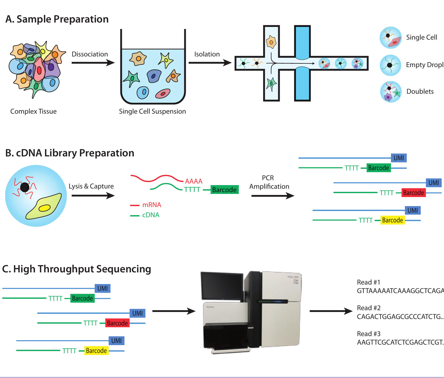
The guide organizes the experimental workflow into three stages:
- Sample preparation. A tissue is dissociated into a single-cell suspension. Microfluidic systems isolate cells, often in oil droplets that also contain a bead carrying a unique DNA barcode.
- Library preparation. Each cell is lysed, its RNA is reverse transcribed into complementary DNA, and cell barcodes and unique molecular identifiers are attached before amplification.
- Sequencing and preprocessing. Sequenced reads are assigned back to their cells, aligned to a reference genome, counted, filtered for technical artifacts, and normalized. The result is a matrix of genes by cells.
Each stage can influence the next one. Dissociation can bias which cells survive, droplets can contain zero or multiple cells, amplification can distort counts, and low-quality cells can introduce misleading structure. The computational pipeline therefore begins with careful quality control rather than immediately looking for biological patterns.
From a matrix to biology
A gene-by-cell matrix is high-dimensional: each gene is a separate axis along which cells may vary. Dimensionality-reduction methods compress that variation into a smaller space that is easier to analyze and visualize. Clustering can then identify groups of transcriptionally similar cells, while differential expression helps find genes that distinguish those groups.
The guide connects those tools to three broad applications: cataloguing cell types in healthy tissue, comparing healthy and diseased cells, and tracking continuous processes such as differentiation.
Place in my research trajectory
This article sits between my earlier experimental work with microfluidic devices and individual cells and my later work on computational models of single-cell data. It gave me a reason to put the whole measurement chain on one page: the physical isolation of cells, the molecular bookkeeping that preserves their identities, and the algorithms that turn sequencing reads into a model of cellular variation.
The specific tools used in single-cell genomics continue to change, but that experimental-to-computational chain is still the mental model I use when approaching the field.
Publication link
- A Beginner’s Guide to Single-Cell Transcriptomics , The Biochemist 41(5), 34-38 (2019)